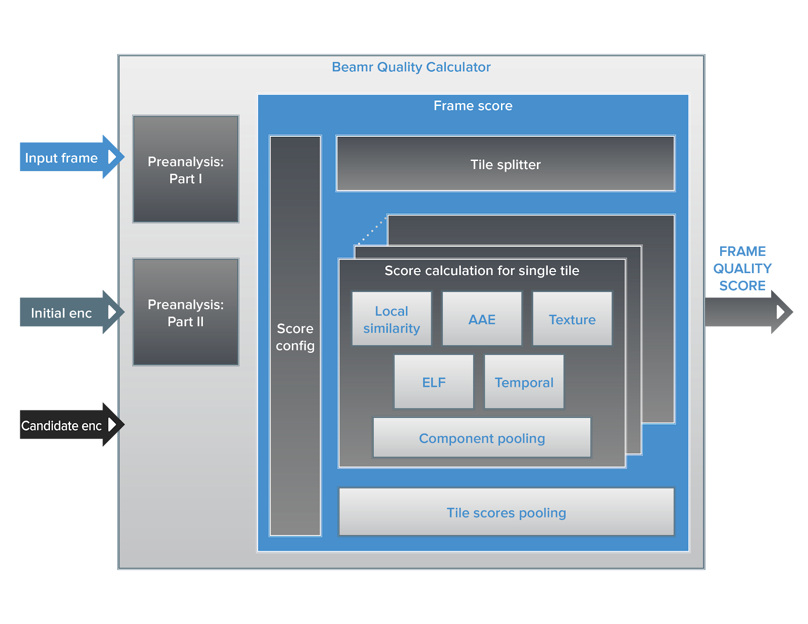
At the heart of Beamr’s closed-loop content-adaptive encoding solution (CABR) is a patented quality measure. This measure compares the perceptual quality of each candidate encoded frame to the initial encoded frame. The quality measure guarantees that when the bitrate is reduced the perceptual quality of the target encode is preserved. In contrast to general video quality measures – which aim to quantify any difference between video streams resulting from bit errors, noise, blurring, change of resolution, etc. – Beamr’s quality measure was developed for a very specific task. It reliably and quickly quantifies the perceptual quality loss introduced in a video frame due to artifacts of block-based video encoding. In this blog post, we present the components of our patented video quality measure, as shown in Figure 1.
Pre-analysis
Before determining the quality of an encoded frame, the quality measure component performs some pre-analysis on the source and initial encoded frames to extract data used in the quality measure calculation and to collect information used to configure the quality measure. The analysis consists of two parts, where part I of the analysis is performed on the source frame and part II of the analysis is performed on an initial encoded frame.

Figure 1. A block diagram of the video quality measure used in Beamr’s CABR engine
The goal of part I of the pre-analysis is to characterize the content, the frame, and areas of interest within a given frame. In this phase, we can determine whether the frame has skin and face areas, rich chroma information typical of 3D animation, or highly localized movement with static background, found in cell animation content. The algorithms used are designed for low CPU overhead. For example, our facial detection algorithm applies a full detection mechanism at scene changes and a unique, low complexity adaptive-tracking mechanism in other frames. For skin detection, we use an AdaBoost classifier, which we trained on a marked dataset we created. The classifier uses YUV pixel values and 4×4 Luma variance values input. At this stage, we also calculate the edge map which we employ in the Edge-Loss-Factor score component described below.
Part II of the pre-analysis is used to analyze the characteristics of the frame after the initial encoding. In this phase, we may determine if the frame has grain and estimate the amount of grain, and use it to configure the quality measure calculation. We also collect information about the complexity of each block, which is indicated, for example, by the bit usage and block quantization level used to encode each block. At this stage, we also calculate the density of local textures in each block or area of the frame, which is used for the texture preservation score component described below.
Quality Measure Process and Components
The quality measure evaluates the quality of a target frame when compared to a reference frame. In the context of CABR, the reference frame is the initial encoded frame and the target frame is the candidate frame of a specific iteration. After performing the two phases of the pre-analysis, we proceed to the actual quality measure calculation, which is described next.
Tiling
After completing the two phases of the pre-analysis stage, each of the reference and target frames is partitioned into corresponding tiles. The location and dimensions of these tiles are adapted according to the frame resolution and other frame characteristics. For example, we will use smaller tiles in a frame which has highly localized motion. Tiles are also sometimes partitioned further into sub-tiles, for at least some of the quality measure components. A quality metric score is calculated for each tile, and these per-tile scores are perceptually pooled to obtain a frame quality score.
The quality score for each tile is calculated as a weighted geometric average of the values calculated for each quality measure component. The components include a local similarity component which determines a pixel-wise difference, an added artifactual edges component, a texture distortion component, an edge loss factor, and a temporal component. We now provide a brief review of these five components of Beamr’s quality measure.
Local Similarity
The local similarity component evaluates the level of similarity between pixels at the same position in the reference and target tiles. This component is somewhat similar to PSNR, but uses adaptive sub-tiling, pooling, and thresholding, to provide results that are more perceptually oriented than regular PSNR. In some cases, such as when pre-analysis determined that the frame contains rich chroma content, the calculation of pixel similarity for chroma planes is also included in this component, but in most cases, only luma is used. For each sub-tile, regular PSNR is calculated. To give greater weight to low-quality sub-tiles, which are located in tiles that have far superior quality, we perform the pooling using only values which are below a threshold that depends on the lowest sub-tile PSNR values. This can happen when there are changes only in a small area, even just a few pixels. We then scale the pooled value using a factor which is adapted according to the level of brightness in the tile, since distortion in dark areas is more perceptually disturbing than in bright areas. Finally, we clip the local similarity component score so that it lies in the range [0,1], where 1 indicates that the target and reference tiles are perceptually identical.
Added Artifactual Edges (AAE)
The Added Artifactual Edges score component evaluates additional blockiness introduced in the target tile compared to reference tile. Blockiness in video coding is a well-known artifact introduced by the independent encoding done on each block. Many previous attempts have been made to avoid this blockiness artifact, mainly using de-blocking filters which are integral parts of modern video encoders such as AVC and HEVC. However, our focus in the AAE component is to quantify the extent of this artifact rather than eliminate it. Since we are interested only in the added blockiness in the target frame relative to the reference frame, we evaluate this component of the quality measure on the difference between the target and reference frames. For each horizontal and vertical coding block boundary in the difference block, we evaluate the change or gradient across the coding block border and compare it to the local gradient within the coding block on either side. For example, for AVC encoding this is done along the 16×16 grid of the full-frame. We apply soft thresholding to the blockiness value, using adaptive threshold values, adapted according to information from the pre-analysis stage. For example, in an area recognized as skin, where human vision is more sensitive to artifacts, we will use tighter thresholds so that mild blockiness artifacts are more heavily penalized. These calculations result in an AAE scores map, containing values in the range of [0, 1] for each horizontal and vertical block border point. We average the values per block border, and then average these per-block-border average values, excluding or giving low weight to block borders with no added blockiness. The value is then scaled according to the percent of extremely disturbing blockiness artifacts, i.e. cases where the original blockiness value prior to thresholding was very high, and finally is clipped to the range [0,1] with 1 indicating no added artifactual edges in the target tile relative to the reference tile.
Texture Distortion
The texture distortion score component quantifies how well texture is preserved in the target tile. Most block-based codecs, including AVC and HEVC, use a frequency transform such as DCT and perform quantization of the transform coefficients, usually applying more aggressive quantization to the high-frequency components. This can cause two different textural artifacts. The first artifact is a loss of texture detail, or over-smoothing, due to loss of energy in high-frequency coefficients. The second artifact is known as “ringing,” and is characterized by the noise around edges or sharp changes in the image. Both these artifacts cause a change in the local variance of the pixel values: over-smoothing causes a decrease in pixel variance, while added ringing or other high-frequency noise, causes an increase in pixel variance. Therefore, we measure the local deviation, in corresponding blocks in the reference and target frame tiles, and compare their values. This process yields a texture tile score in the range [0,1] with 1 indicating no visible texture distortion in the target image tile.
Temporal consistency
The temporal score component evaluates the preservation of temporal flow in the target video sequence compared to the temporal flow in the reference video sequence. This is the only component of the quality measure that also requires the preceding target and reference frames to be leveraged. In this component, we measure two kinds of changes: “new” information introduced in the reference frame which is missing in the target frame, and “new” information in target frame where there was no “new” information in the reference frame. In this context, “new” information refers to information that exists in the current frame but doesn’t exist in the preceding frame. We calculate the Sum of Absolute Differences (SAD) between each co-located 8×8 block in the reference frame and the preceding reference frame, and the SAD between each co-located 8×8 block in the target frame and the preceding target frame. The local (8×8) score is derived from the relation between these two SAD values, and also according to the value of the reference SAD, which indicates whether the block is dynamic or static in nature. Figure 2 illustrates the value of the local score for different combinations of the reference and target SAD values. After all local temporal scores are calculated, they are pooled to obtain a tile temporal score component in the range [0,1].

Figure 2. local temporal score as a function of reference SAD and target SAD values
Edge Loss Factor (ELF)
The Edge Loss Factor score component reflects how well edges in the reference image are preserved in the target image. This component uses the input image edge map, generated during part I of the pre-analysis. In part II of the pre-analysis, the strength of the edge at each edge point in the reference frame is calculated, as the most substantial absolute difference between the edge pixel value and its 8 closest neighbors. We can optionally discard pixels which are considered false edges, by comparing the reference frame edge strength of the pixel to a threshold, which can be adapted, for example, to be higher in a frame which contains film grain. Once values for all edge pixels have been accumulated the final value is scaled to provide an ELF tile score component, in the range [0,1] with 1 indicating perfect edge preservation.
Combining the Score Components
The five tile score components described above are combined into a tile score using weighted geometric averaging, where the weights can be adapted according to the codec used or according to the pre-analysis stage. For example, in codecs with good in-loop deblocking filters we can lower the weight of the blockiness component, while in frames with high levels of film grain (as determined by the pre-analysis stage) we can reduce the weight of the texture distortion component.
Tile Pooling
In the final step of the frame quality score calculation, the tile scores are perceptually pooled to yield a single frame score value. The perceptual pooling uses weights which are dependent on importance (derived from the pre-analysis stages, such as the presence of face and/or skin in the tile), and on the complexity of blocks in the tile compared to average complexity of the frame. The weights are also dependent on tile score values – we give more weight to low scoring tiles, in the same way, human viewers are drawn to quality drops even if they occur in isolated areas.
Score Configurator
The score configurator block is used to configure the calculations for different use cases. For example, in implementations where latency or performance are tightly bounded, the configurator can apply a fast score calculation which skips some of the stages of pre-analysis and uses a somewhat reduced complexity score. To still guarantee a perceptually identical result, the score calculated in this fast mode can be scaled or compensated to account for the slightly lower perceptual accuracy, and this scaling may in some cases slightly reduce savings.
To learn more about CABR, continue reading “A Deep Dive into CABR, Beamr’s Content-Adaptive Rate Control.”
Authors: Dror Gill & Tamar Shoham